What is the Hybrid Lognormal Distribution?

Abstract

This paper reports on a case study in radiation protection, revealing that the statistical phenomena observed in the dose distribution of workers under dose reduction management exhibit an intriguing new probability distribution. This distribution unifies the lognormal and the normal distributions—previously considered distinct—by replacing the upper tail of the former with that of the latter. It is adjusted by the parameter ρ from the former (ρ → 0) to the latter ( → ∞), allowing for an accurate analysis of the statistical phenomena existing between the two. This is the “hybrid lognormal (HLN) distribution,” defined by the hybrid transformation hyb(ρX) = ln X + X, which replaces the logarithmic transformation ln X. The stimulus η = Δhyb(ρX) yields the increment ΔX = ηX/(1+ρX). Interpreting the numerator as the risk increment and the denominator as the risk reduction (achieved through feedback control), this equation represents the simplest risk management principle. The hybrid transformation is visualized as a hybrid scale (HS) consisting of a logarithmic scale and a linear scale, demonstrating its utility in evaluating the effectiveness of risk management. We discuss the background of this case study, the generation mechanism and statistical characteristics of the HLN distribution, application examples, as well as its position within the context of probability distributions and the applicability of the hybrid scale to case studies.

Introduction

In the fields of clinical and medical case studies, evaluating the effectiveness of health risk management associated with any form of harmful exposure is a critical issue. In the field of radiation protection, the distribution characteristics of annual individual doses from occupational exposure—which are managed and reduced in accordance with legal standards—are regarded as a fundamental basis for comprehensively evaluating the effectiveness of protection [1]. Interest in individual dose distributions focuses on the characteristics of the probability distribution obtained by evaluating the effective dose corresponding to the lifetime health detriment calculated for an exposed population. The objective is to determine the necessary increase in dose for human activities while ensuring that health risks are kept below tolerable levels and managed in accordance with the “As Low As Reasonably Achievable (ALARA)” principle. In the early 1980s, the “hybrid lognormal (HLN) distribution” was proposed as a probability distribution suitable for this task [2–7].

The HLN distribution is useful for examining the statistical distribution characteristics of health risk reduction effect under specific conditions using the hybrid scale consisting of logarithmic and linear scales that visualize the hybrid transformation. This transformation provides the simplest risk management principle rationally combining risk increase and risk reduction based on feedback control. Furthermore, since the HLN distribution is a hybrid form (utilizing the hybrid transformation) that combines the characteristics of both distributions, with the upper tail of the lognormal distribution transitioning to that of the normal distribution, it provides a more rigorous and useful analytical method for addressing the issue raised by Masuyama [8] regarding whether to use the normal distribution or the log-normal distribution when analyzing measured data such as blood concentrations.

This paper focuses on these perspectives and, as a case study, describes the background leading to the proposal of the HLN distribution, its characteristics and generation mechanism, and practical application examples. It also briefly discusses the historical background, the potential for future development of the proposed distribution, and the wide-ranging usefulness of hybrid scales.

Motivation for the HLN distribution model

The annual individual dose distribution model was developed by the United Nations Scientific Committee on the Effects of Atomic Radiation (UNSCEAR) [9] to establish a dose limit system in accordance with the ICRP’s 1977 Recommendations. Using a large number of dose statistics from various countries, UNSCEAR constructed a reference dose distribution based on a lognormal distribution (arithmetic mean 5 mSv; upper-tail probability Q(>50 mSv) = 0.001). The ICRP [10] adopted this distribution model to establish dose limits that meet safe industrial risk levels. On the other hand, when applying a lognormal distribution to annual individual dose statistics for occupational exposure in the nuclear field, a phenomenon was observed in which the upper tail of the distribution was skewed toward lower doses [9,11]. This was interpreted as resulting from dose reduction management measures implemented mid-year to ensure compliance with dose limits.

Since the skewness of the upper-tail is important for accurately analyzing fluctuations in high dose values near dose limits, following the ICRP’s 1977 recommendations, Warman et al. [12] reported that a two-component mixed log-normal distribution—which models the upper-tail skewness with a separate log-normal distribution—is effective. On the other hand, based on our experience in constructing a distribution of individual doses for the general public (mean 1.7 mSv, probability Q(>5 mSv) = 0.001 to 0.000001) in accordance with U.S. Federal Radiation Protection Guidance using a lognormal distribution [13], we concluded that it was necessary to fundamentally elucidate the mechanism by which dose reduction management causes skewness in the upper tail of the lognormal distribution.

A detailed investigation of this statistical phenomenon revealed that the skewed upper tail exhibits characteristics of a normal distribution. Therefore, we constructed a probability distribution called the “hybrid lognormal distribution” by replacing the logarithmic transformation ln X with the hybrid transformation hyb(ρX) = ln ρX + ρX, where ρX is a dimensionless quantity defined as the product of the dose reduction coefficient ρ (mSv⁻¹) and the dose X (mSv) [2,4]. Since this probability distribution is more complex than the log-normal distribution and requires numerical calculations to determine its statistical parameters, we developed a computational package for dose distribution analysis [2,3].

Practical applications for occupational exposure

Using the dose distribution analysis software package, we were able to verify its consistent and comprehensive applicability of the HLN distribution to the analysis of downward trends in dose distributions from 1960 to 1985—conducted by the EPA to revise the Federal Radiation Protection Guidance for occupational exposure—and to the detailed 1980 assessment based on that analysis [14,15]. The HLN distribution made it possible to improve the accuracy of the 1980 assessment—which was based on existing data that was partially uncertain—by comparing the 1985 dose distribution forecast, derived from nationwide downward trends reconstructed from dose distributions by calendar year and across all industrial sectors in the United States, with the same forecast under conditions conforming to the 1977 ICRP recommendations. Furthermore, in the 1980 assessment, the applicability of the HLN distribution was verified by gender and age group.

Furthermore, as a case study analyzing the effectiveness of dose reduction management based on the ALARA principle at radiation work sites using the HLN distribution, we demonstrated that it is possible to accurately evaluate the differences in reduction measures between high-dose-rate and low-dose-rate areas for a series of special radiation operations at the JRR-2 and JRR-3 research reactors [16]. Both the distribution of daily doses for individual workers and the pooled daily dose distribution for all workers followed an HLN distribution under access control criteria; furthermore, the individual cumulative doses among workers followed an HLN distribution with the parameter ρ corresponding to the management target value for the work period. Thus, it was found that the HLN distribution can be applied to the analysis of dose distributions—ranging from daily individual doses to cumulative individual doses—that demonstrate dose reduction effects reflecting both management target values and the ALARA principle. Furthermore, the Canadian National Dose Registry has implemented an update to the dose analysis software package we developed [3] that incorporates the maximum likelihood estimation method [17].

The generation mechanism of the HLN distribution

In paragraphs 20 and 32 of Annex H to the 1982 UNSCEAR Report [18], it was pointed out that the hybrid lognormal distribution [4] is likely a more suitable method for representing observed distributions because it incorporates the constraining function of the feedback mechanism governing doses approaching dose limits.

We applied engineering feedback control, which represents the “chain of information transmission and feedback” proposed by cybernetics pioneer Wiener [19], to derive the increment ΔX_j = η_jX_j-1 /(1+ρX_j-1) for the HLN distribution from the increment ΔX_j = η_jX_j-1 of the stochastic process generating the lognormal distribution proposed by Kapteyn [20]. Specifically, the dose reduction control measure, which replaces η_j with η_j − ρΔX_j via the feedback coefficient ρ, results in the increment being reduced to 1/(1 + ρX_j-1) [5]. As a result, based on the Central Limit Theorem, the sum of random reaction intensities A_n = Σ η_j = Σ Δhyb(ρXj) converges to a normal distribution. The right-hand side becomes an asymptotic definite integral over the finite time interval [0, T]: ∫ d hyb(ρx) = hyb(ρXT) − hyb(ρX0). Therefore, hyb(ρXT) follows a normal distribution, and a HLN distribution is generated for X_T.

From the perspective of statistical theory, since the increment ΔX_j = η_jX_j-1 /(1+ρX_j-1) incorporates a feedback mechanism based on past information, a proof of the generation mechanism based on the martingale central limit theorem was provided [6] (see Appendix). The term “hybrid lognormal distributions” appears on page 71 of the Supplement Volume to the Encyclopedia of Statistical Science edited by Kotz and Johnson [7].

The simplest principle of risk management

The HLN-type increment ΔX_j = η_jX_j-1 /(1+ρX_j-1) is smaller than the LN-type increment ΔX_j = η_jX_j-1 [5] due to the denominator term corresponding to feedback control. This reduction reflects the most rational reduction mechanism observed in nature [21,22]. A typical example is elucidating the suppression mechanisms governing neutron excess (NE) in stable nuclei through element synthesis processes such as supernova explosions.

NE in stable nuclei increases with increasing proton number Z in accordance with the balance between the Coulomb force and the nuclear force, and ΔNE(Z)/ΔZ = ηNE(Z) is determined by the reaction coefficient η. On the other hand, this increase is suppressed by the constraint that the mass of a neutron is slightly greater than that of a proton, as well as by the energy equation E = mc², which acts through the feedback coefficient ρ. Consequently, ΔNE(Z)/ΔZ = ηNE(Z)/(1 + ρNE(Z)). This can be expressed by the linear regression equation hyb(ρNE) = α + βZ, where ρ is solved nonlinearly. Using the 2018 edition of the “JAEA Chart of the nuclides,” we verified this equation for 271 nuclides with half-lives T1/2 ≥ 5 × 108 years and NE > 0; the R² value was 0.9606, confirming the validity of this equation [23]. Furthermore, for the 286 nuclides including those with NE(Z) ≤ 0, when the equation was expressed as hyb(ρ(NE+a)), $\widehat{a}$ = 3.4 ± 1.2, and the R² value was 0.9863.

The HLN increment ΔX_j = η_jX_j-1 /(1+ρX_j-1) thus reveals the natural phenomenon underlying the “risk control” inherent in stable atomic nuclei. Therefore, the most concise mathematical model for health risk management must, at a minimum, include a mechanism that reasonably balances the terms that increase risk with those that suppress it, and the HLN increment satisfies this functional requirement.

Properties of the HLN distribution

The HLN distribution is a probability distribution for a positive variable X such that the hybrid transformation hyb(ρX), where ρ is a positive constant, follows a normal distribution N(μ, σ₂) with mean μ = E[hyb(ρX)] and variance σ₂ = V[hyb(ρX)]. The hybrid function s = hyb(t) = ln t + t and its inverse function cyb(s) = cyb(hyb(t)) = t are indispensable for the numerical calculation and theoretical analysis of various statistical quantities of the HLN distribution (−∞ < s < ∞; 0 < t < ∞). These functions correspond, respectively, to the logarithmic function s = ln t and the exponential function t = exp(s) of the lognormal distribution.

Research on the HLN distribution consists of the interplay between the mathematical properties of the hybrid function and normal theory; in accordance with this, along with the constrained lognormal theory defined for positive random variables, useful moment distributions are defined. This is useful for analyzing collective dose distributions in occupational exposure. Just as a random variable following a lognormal distribution is called a Λ-variate, a random variable X following a HLN distribution is called an Ω-variate and is denoted as X ~ Ω(ρ, μ, σ₂). From the definition of the HLN distribution, hyb(ρX) ~ N(μ, σ₂), and the following relationship holds for Z ~ N(0,1):

$=\frac{hyb\left(\rho X\right) - \mu }{\sigma }orhyb\left(\rho X\right)=\mu + \sigma Z$ (1)

The hybrid transformation hyb(ρX) asymptotically converges to ln X as ρ → 0 and asymptotically converges to X (>0) as ρ → ∞. Therefore, when R = ρX ≤ 0, where the cumulative distribution function is P(Z ≤ −μ/σ) = Φ(−μ/σ), X⁺(R) ~ N(μ, σ₂) is defined as the positive normal distribution (PN distribution), where the transformation X⁺(R) is given by the following:

X⁺(R) = max(0+, R | 0 < 0+ < ε, (ε → 0); −∞ < R < ∞) (2)

Since R = ρX ≤ 0 belongs to the cumulative distribution function of P(Z ≤ −μ/σ), it is compressed into a neighborhood of 0+. Therefore, unlike the truncated normal distribution, the PN distribution has a cumulative distribution function Φ((x − μ)/σ) for x > 0. A random variable X following the PN distribution is called a Ψ-variable and is denoted as X ~ Ψ(μ, σ₂).

An Ω-variate X^Ω that follows the HLN distribution asymptotically approaches an Λ-variate X^Λ that follows a log-normal (LN) distribution as ρ → 0 and asymptotically approaches a Ψ-variate X^Ψ that follows a PN distribution as ρ → ∞. The Ω-variate X^Ω of the HLN distribution itself approximates the Λ-variate X^Λ in the region where | ln ρX | >> ρX, i.e., 0 < ρX << 1, and approximates the Ψ-variate X^Ψ in the region where | ln ρX | << ρX, i.e., 1 << ρX < ∞; In the intermediate region where 0.01 ~ 0.1 ≤ ρX ≤ 5 ~ 20, the Ω-variate X^Ω exhibits transition characteristics where it continuously shifts from the X^Λ approximation to the X^Ψ approximation. For convenience, the entire Ω-variate X^Ω is composed of the following regions:

{X^Λ approximation, X^Ω transition, X^Ψ approximation} (3)

These characteristics demonstrate that, by varying the positive ρ, a given data range (x^min, x^max) is uniquely represented within the framework of the Ω-variate X^Ω by either the X^Λ approximation, the X^Ω transition, or the X^Ψ approximation.

The cumulative distribution function of the HLN distribution is Ω(x) = Φ(z) = Φ[(hyb(ρx) − μ)/σ], and the probability density function is derived as follows using the expression ω(x)dx = φ(z)dz:

$=\frac{\text{hyb}\left(\rho X\right)- \mu }{\text{σ}}or\text{ hyb}\left(\rho X\right)=\mu + \sigma$ (4)

The 100Q percentile is denoted as ZQ, and $\text{hyb}\left(\rho x_Q\right)=\mu +\sigma z_Q;$ therefore, the median is given by which $\text{hyb}\left(\rho \tilde{x}\right)=\mu ,$ is equivalent to $\tilde{x}={\rho }^{-1}\text{cyb}\left(\mu \right).$ The mode x^m is unimodal except under the bimodality condition where μ > 3 - ln 3 and ${\sigma }_a^2\left(\mu \right)<{\sigma }^2<{\sigma }_b^2\left(\mu \right)$ [3,6]. Expressed as the jth-order moment ${\rho }^{-j}{\varphi }_j$ around the origin, the arithmetic mean is ${\rho }^{-1}{\varphi }_1,$ and the standard deviation is ${\rho }^{-1}{\left({\varphi }_2-{\varphi }_1^{ 2}\right)}^{1/2},$ the geometric mean ${\mu }_g={\rho }^{-1}\text{exp}\left(\mu -{\varphi }_1\right),$ and the geometric standard ${\sigma }_g=\text{exp}\left[{\left\{{\beta }^2+{\sigma }^2\left(1-2\partial {\varphi }_1/\partial \mu \right)\right\}}^{1/2}\right].$

The double-logarithmic plot of skewness versus kurtosis, which characterizes the shape of a distribution, forms a right-ascending straight line for the LN distribution. When the kurtosis on the x-axis is fixed, the plot for the HLN distribution lies above the straight line on the side where skewness increases, and its maximum range varies depending on the parameters (µ, σ) such that it asymptotically approaches the plot for the PN distribution (see [6] for a detailed figure).

The hybrid mean $m_{H^{*}}$ is the HLN median defined as $\text{hyb}\left(\rho m_{H^{*}}\right)=E\left[\text{hyb}\left(\rho X\right)\right]=\mu$ or $m_{H^{*}}={\rho }^{-1}\text{cyb}\left(\mu \right).$

Using by $E\left[\text{hyb}\left(\rho X\right)\right]=E\left[\text{ln }\rho X+\rho X\right]=\text{ln }\rho m_G+\rho m_P$

$\therefore m_{H^{*}}={\rho }^{-1}\text{cyb}\left(\text{ln }\rho m_G+\rho m_P\right)$ (8)

Also $\rho =\left(\text{ln }{m}_{H^{*}}/m_G\right)/\left(m_P-m_{H^{*}}\right)$ is obtain from the equation of $\text{ln }\rho m_{H^{*}}+\rho m_{H^{*}}=\text{ln }\rho m_G+\rho m_P.$ The hybrid mean $m_{H^{*}}$ approximates the geometric mean m_g when $\left|\text{ln }\rho m_G\right|\gg \rho m_P$ and approximates the positive arithmetic mean m_p when $\text{ln }\rho m_G\ll \rho m_P.$ The hybrid standard deviation $s_{H^{*}}$ is defined as $s_{H^{*}}={\rho }^{-1}\text{cyb}\left(\sigma \right)$ from ${\left\{\text{hyb} \left(\rho s_{H^{*}}\right)\right\}}^2=V\left[\text{hyb}\left(\rho X\right)\right]={\sigma }^2.$ The hybrid mean and hybrid standard deviation are fundamental statistics for the HLN distribution.

Practical application examples

Numerous examples of the application of the HLN distribution can be found across various fields. With regard to epidemiological cohorts, the statistics for whole-body external dose (Gy) in Table 11 and the statistics for Pu body burden (kBq) in Table 12 of the Mayak Workers Cohort (MWC) [24] are both fitted to the HLN distribution with R² > 0.99. Furthermore, the dose statistics for LSS solid cancer incidence (1985–2009) in Table 3 [25] fit the HLN distribution with R² > 0.999 for both males and females. For males, the estimated mean for doses of 0.005 or higher is 0.2191 Gy. Excluding the control group (< 0.005 Gy), for the HSB distribution hyb(ρ(X−a)/(b−X)) ~ N(µ, σ₂) with assumed parameters a = 0.005 Gy and b = 6 Gy, R² = 0.9998 for male, yielding an estimated mean of 0.2188 Gy; both values agree with 0.22 Gy. Therefore, depending on the need to include the lower limit a or/and upper limit b, the HLN4 distribution hyb[ρ(X−a)] ~ N(µ, σ₂), the HSB4 distribution hyb[ρX/(b−X)] ~ N(µ, σ₂), or the HSB distribution hyb[ρ(X−a)/(b−X)] ~ N(µ, σ₂) are applied, depending on the need to include these limits. Note that the HSB distribution is also an abbreviation for the hybrid S_B distribution, which is derived from the Johnson S_B (JS_B) one ln[(X−a)/(b−X)] ~ N(µ, σ₂) by incorporating feedback control [26].

U.S. occupational exposure statistics are often well approximated by the HLN distribution [27]; however, Figure 1 shows an example where the HLN distribution should be applied to the dose range a < D < b. Figure 1 shows the dose histogram (Figure 5) [28] presented under the premise that “not all dose distributions follow the HLN distribution”; for each upper limit Di of the dose bins, Φ(Zi) = P(D ≤ Di) was calculated, and the HLN distribution was fitted using the regression equation hyb[ρ(Di−a)/(b−Di)) = µ + σ Zi. This allows for easy parameter estimation.

Figure 1: HLN plot assuming a < D < b for Kola NPP 2016 [28].

Figure 1 confirms that the 2016 dose distribution at the Kola NPP can be modeled using the HSB-type of HLN distribution with R² = 0.993. Figure 2 shows the HSB4-type of HLN distribution with R² = 0.9983 of the dose distribution for Korean NPPs in 2017 [29] (see upper right panel). The difference in fit between the HLN distribution and the HSB4 distribution is useful for investigating differences in dose reduction effects based on two-stage dose constraints set at the 80th and 90th percentiles of the 20 mSv/ dose limit. In this case, although a slight difference between the two distributions is observed in the lower range, the difference in estimates such as the mean is small. When this difference is significant, the application of the HSB-type becomes effective.

Figure 2: Probability plots of Korean-NPPs dose statistics in 2017 [29].

Discussion

The discussion on the HLN distribution will focus, on the one hand, on its role in probability and statistics, and, on the other hand, on the practical application of the hybrid scale derived from the HLN distribution.

Its role in probability and statistics

Approximately 100 years after Galton [30] proposed the log-normal distribution based on the geometric mean as a counterpart to the normal distribution based on the arithmetic mean, a statistical phenomenon in which these two important probability distributions merge was identified in the field of radiation protection practice as the hybrid lognormal distribution. The advantage of combining these two distributions lies in providing a method for accurately analyzing statistical phenomena in which multiplicative and additive variations coexist simultaneously. This is one of the important roles of the hybrid lognormal distribution in the field of probability and statistics.

When considering multiplicative variation (proportional variation) as measurement error, the solution obtained using the least squares method or the maximum likelihood method is the geometric mean; when considering additive variation as measurement error, the solution is the arithmetic mean. When both types of variation coexist in the ratio ρ, the best approach for converting multiplicative variation into additive variation is to apply a logarithmic transformation and combine them under conditions that allow for addition, resulting inevitably in the hybrid transformation hyb(ρX) = ln ρX + ρX.

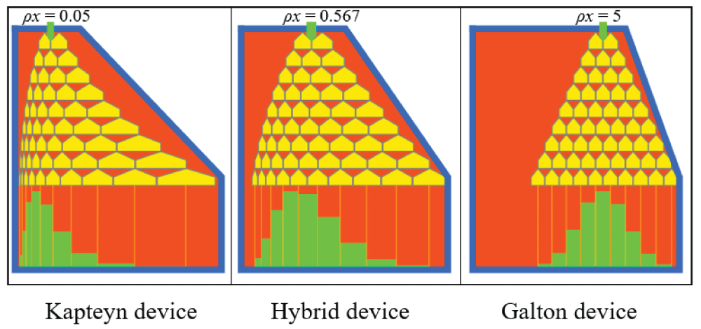
In a Galton device that forms a Gaussian curve, small balls falling from above are deflected left and right by multi-stage pegs arranged at equal intervals; as a result, despite traveling through complex and varied paths, the cumulative height of the balls accumulating in the troughs of equal width prepared at the bottom approaches a Gaussian distribution. A Kapteyn-analogue device forms an LN curve when the width of the left-right branching caused by a peg increases proportionally to the distance of that peg from the leftmost reference line, and the width of the trough in the lower section correspondingly increases in proportion to the distance from the left end. The left-right branching width ΔX at peg position X is expressed as ΔXG = ±ηG for the Galton apparatus and ΔXK = ±ηKXK for the Kapteyn apparatus; this corresponds to ΔlnXK = ±ηK. When the left-right branching widths of both devices are equal to the reaction intensity ±η = ±ηK ± ρηG, a hybrid device is obtained such that ΔlnXK +ρΔXG = ±η, leading to Δln ρX + ΔρX = Δhyb(ρX) = ±η. This increment is ΔX= ±ηX/(1+ρX). At this point, an HLN curve is formed in the troughs of hybrid width located in the lower section.

To summarize the above, it can be concluded that for the three curve-forming devices, the distance from the left end of the lower trough forms an arithmetic sequence in the Galton device, a geometric sequence in the Kapteyn device [31], and a hybrid sequence integrating both arithmetic and geometric sequences in the hybrid device that combines the two. Expanding on the concept that Pascal [32] called the “arithmetic triangle,” this corresponds to the Galton device; the “geometric triangle” corresponds to the Kapteyn device; and the “hybrid triangle” corresponds to the HLN curve-generating device (Figure 3).

Figure 3: The HLN curve-generating devices (ρx: distance from left).

Another important role of the HLN distribution is that it introduced feedback control into probability distributions. Specifically, it incorporated the engineering concept of feedback control—which represents the “chain of information transmission and feedback” proposed by Wiener [19], a pioneer in cybernetics—into probability distributions. Mathematically, this feedback control is modeled as a hybrid transformation which is the sum of log-term and linear term. As a result, by replacing the logarithmic transformation with a hybrid transformation for distributions other than the normal distribution—such as the hybrid Pareto distribution, hybrid Weibull distribution, hybrid Fréchet distribution, hybrid logistic distribution, and hybrid uniform distribution—it is suggested that these distributions could be applied to uncertainty analysis in the safety assessment of long-term radioactive waste disposal.

In probability distributions based on the HLN model, the degree to which feedback effects manifest is reflected in the parameters and can be visualized. Since modern society has a complex structure with various goal-oriented elements, the fact that the hybrid lognormal distribution translates into a normal distribution through a hybrid transformation not only allows us to leverage the body of knowledge in normal distribution theory but also, because this probability distribution is reproducible, provides the capability to aggregate control results derived from different goal-oriented approaches by utilizing this reproducibility. Therefore, it is possible to quantify the aggregate effect of complex, uncertain factors related to health risks as the parameter ρ. At the very least, the benefits of aggregating the uncertain and complex phenomena observed in case studies—achieved by integrating the log-normal and normal distributions and introducing feedback functionality into the probability distribution—into the parameter ρ should be further investigated in future research.

Practical application of hybrid scales

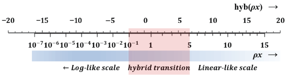
A hybrid scale (HS) is a continuous integration of logarithmic and linear scales, as shown in Figure 4, by the appropriate values of ρx marked below the evenly spaced number lines of hyb(ρx). In Figure 4, the hybrid scale approximates a logarithmic scale when ρx < 0.1 and a linear scale when ρx ≥ 5. The intermediate range of 0.1 ≤ ρx ≤ 5 represents the HLN transition region, where both promoting and inhibiting factors contribute. Since hyb(0.1) = -2.2 and hyb(5) = 6.6, the HLN transition region is defined as -2.2 ≤ hyb(ρx) ≤ 6.6. For the range of measured data (x^min, x^max), if ρx^max < 0.1 or hyb (ρx^max) < −2.2, the data is judged to follow an LN distribution; conversely, if x^min > 5 or hybrid(ρx^min) > 6.6,the data is judged to follow a PN distribution (normal distribution). In all other cases, the data is judged to follow an HLN distribution. By estimating ρ based on the measured data and observing whether the ρx_i or hyb(ρx_i ) values fall within the HLN transition region, it is possible to evaluate the effectiveness of reduction control measures.

Figure 4: Hybrid Scale (HS) corresponding to the hybrid transformation.

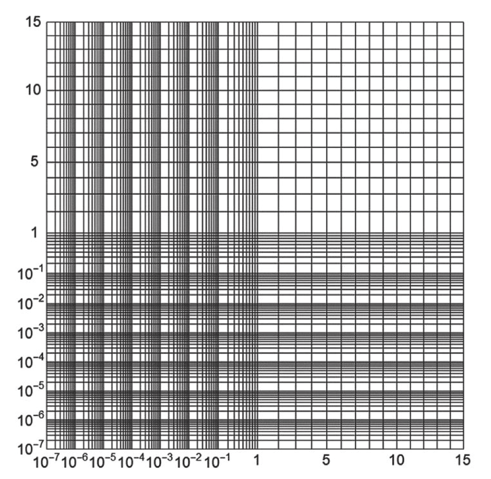
When hybrid scales are applied to the vertical and horizontal axes as Figure 5, and the hybrid scale is viewed as consisting of three components—{logarithmic scale approximation, hybrid transition, linear scale approximation}—the 3×3 combinations result in the formation of five types of hybrid graph paper between standard graph paper (linear on both axes), semi-log graph paper (two types with one axis logarithmic), and log-log graph paper (both axes logarithmic).

Figure 5: Hybrid-Hybrid Graph Paper (τx, νy)

In the region on the right (vertical: hybrid scale; horizontal: linear scale), the survival S(D) of X-ray-irradiated cells is represented by a decreasing linear graph of dose D, hyb(ρS(D)) = hyb(ρ) − λD, where λ is the cell inactivation constant, and ρ is the feedback repair effect, such that ΔS(D)/ΔD = −λS(D)/(1+ρS(D). In the lower region (vertical: logarithmic scale; horizontal: hybrid scale), the logarithm of the cancer incidence rate per surviving cell, F(D) = I(D)/S(D), is represented by the linear graph of the hybrid transformation of dose D: ln(F(D)) = α + βhyb(τX). Here, α is the intercept, β is the slope, and τ is the coefficient (Gy⁻¹) at which the power-law increase of τD transitions to an exponential increase. Based these two linear equations, the Generalized HS (GHS) model is reconstructed as a dose-response relationship, including the probability of survival of transformed cells, in the cancer incidence function I(D) = F(D)S(D). The GHS model, which applies the hybrid-hybrid graph paper, can be applied to the dose-response relationships of LSS and mouse cancer incidence [33].

The graph of chromosome aberration frequency is displayed as a straight line at various regions on hybrid-hybrid graph paper [34]. There are various other applications, and the method is expected to be applied to case studies and research.

Conclusion

This paper discusses the characteristics and applications of the hybrid lognormal (HLN) distribution, which was derived by incorporating the feedback effects of dose reduction management into the generation mechanism of the lognormal distribution. Since the HLN distribution is a new probability distribution, statistical calculation codes for dose distribution analysis have been developed. As examples of its application, this paper describes the use of these codes to analyze the nationwide occupational exposure dose statistics for 1960–1985 compiled by the Environmental Protection Agency (EPA), an analysis of dose reduction effects based on federal guidelines, and the formulation of a dose reduction plan for a research reactor at the Japan Atomic Energy Agency (JAEA). It was noted that, 100 years after the lognormal distribution was proposed for measured values to which the normal distribution does not apply, the HLN distribution plays an important role as a probability distribution that can be applied even when measured values from both distributions coexist in any proportion. At the same time, by incorporating feedback control into a synergistic stochastic process, the concepts of HLN increment—which quantifies the effectiveness of reduction management—and the corresponding hybrid transformation were introduced. This provides a principle for achieving a “balance between increase and suppression,” and it was demonstrated that hybrid scales are useful for visualizing this balance. Furthermore, it was demonstrated that graph paper with hybrid scales applied in two dimensions can be widely used as a method that brings new extensions to regression analysis, such as the continuous extension of power laws and exponential functions. Since the HLN distribution is expected to lead to advancements not only in probability theory and statistics but also in a wide range of other fields, its application in various disciplines—including this basic research—is anticipated in the future.

Appexdix

HLN Generation Mechanism [6].

Following Kapteyn [20], we view the growth process of a biological organ as a stochastic stimulus-response process consisting of n stages. We assume that an organ of size X₀ = X_0|n grows to X_j|n after j stages and reaches X_T = X_n|n after n stages. This stochastic process continues for a finite time interval [0, T], and the hypothetical number of stages n is assumed to be arbitrarily large. Hereinafter, unless otherwise specified, the subscript j|n is written simply as j.

Kapteyn’s model assumes that the stimulus variable at the jth stage is η_j, and that the response ΔX_j = X_j − X_j-1 to this stimulus is expressed as the product of the previous organ size X_j-1 and η_j. Here, to prevent the final organ size X_T from becoming excessive, we assume that the effective stimulus η_j is reduced to η_j′, thereby reducing the response quantity to ΔX_j ′. This reduction is considered to result from feedback with a positive constant ρ. That is, we assume that ΔX_j ′ = η_j′X_j-1 and η_j′ = η_j − ρΔX_j ′ hold simultaneously. Furthermore, assuming that feedback also operates in the preceding stage, let

ΔX_j ′ = η_j′X_j-1′, so that

ΔX_j ′ = η_jX_j-1 ′/(1+ρX_j-1′). (A-1)

Here, we solve Eq. (A-1) for η_j and compute the sum:

An(t) = ∑* η_j|n = ∑* (1/X_j-1′ + ρ) ΔX_j ′, (A-2)

where, ∑* indicates that the sum is taken from j = 1 to [nt | T].

We now make the following assumptions:

[0] The number of stages n in the growth process can be made arbitrarily large.

[1] $>xmlns=\text{'}http://www.w3.org/1998/Math/MathML\text{'}>\underset{1\le j\le n}{\max }{\eta }_{j|n}$ converges in the limit to 0 as n increases.

[2] The expected value M_n(t) of A_n(t) converges in probability to a certain constant function M(t).

[3] The variance V_n(t) of A_n(t) converges in probability to a certain constant function V(t).

For example, if n is fixed and η_j|n follows an independent identically distributed (i.i.d.) distribution with mean c₁/n and variance $>\; xmlns=\text{'}http://www.w3.org/1998/Math/MathML\text{'}>c_2{}^2/n$ (where c₁ and c₂ are constants independent of n), then by setting M(t) = c₁t/T and $>\; xmlns=\text{'}http://www.w3.org/1998/Math/MathML\text{'}>V\left(t\right)=c_2{}^{2}t/T$ , conditions [1] – [3] are satisfied. Under the above conditions, A_n(t) − M_n(t) is a martingale, and by the martingale central limit theorem (e.g., Gill [34], p. 445), the limit distribution of An(t) is the normal distribution. Furthermore, from Eq. (A-2), we have ΔX_j ′ < η_j/ρ, and considering condition [1], An(t) converges as follows, where hyb(t) = ln t + t:

$>\; xmlns=\text{'}http://www.w3.org/1998/Math/MathML\text{'}>{\int }_{X_0}^{X_T}\left(\frac{1}{X}+\rho \right)dX=\text{hyb}\left(\rho X_T\right)-\text{hyb}\left(\rho X_0\right)$ (A-3)

Ultimately, it has been proven that X_T follows the HLN distribution.

References

1. 1990 recommendations of the ICRP. ICRP Publ 60. Ann ICRP. 1991;21(1‑3).

2. Kumazawa S, Shimazaki J, Numakunai T. Computational algorithms for the hybrid lognormal distribution (in Japanese). Proc 2nd Symp Appl Stat. Tokyo; 1980 Oct 25. Abstracts D3‑1–D3‑10. Jpn Soc Appl Stat.

3. Kumazawa S, Shimazaki J, Numakunai T. Numerical calculation methods relating to hybrid lognormal distributions (in Japanese). JAERI‑M 82‑035. 1982 Apr.

4. Kumazawa S, Numakunai T. A new theoretical analysis of occupational dose distributions indicating effects of dose limits. Health Phys. 1981;41(3):465‑75.

5. Kumazawa S. The generation mechanism of the hybrid lognormal distribution and its engineering applications (in Japanese). IEICE (A). 1982;J65‑A(2):201‑2.

6. Kumazawa S, Ohashi Y. Hybrid lognormal distribution and its application (in Japanese). Jpn J Appl Stat. 1986;15(1):1‑14.

7. Kotz S, Johnson NL. Encyclopedia of statistical sciences. Supplement Vol. New York: John Wiley & Sons; 1989.

8. Masuyama G. To all students who don’t want to end up as computer parts (in Japanese). Tokyo: Misuzu Shobo; 1987. ISBN: 4‑622‑02491‑8.

9. Sources and effects of ionizing radiation. 1977 report of United Nations Scientific Committee on the Effect of Atomic Radiation. Annex E. United Nations; 1977.

10. 1977 recommendations of the ICRP. ICRP Publ 26. Ann ICRP. 1977;1(3).

11. Gale HJ. The lognormal distribution and some examples of its application in the field of radiation protection. AERE‑R4736. 1965.

12. Warman EA, McMellon RL, Cardito JM. Occupational radiation: exposure reduction technology planning study. US EPRI NP‑1962. 1981.

13. Kumazawa S. The relationship between average and maximum doses within the lognormal population (in Japanese). Proc Atomic Energy Soc Jpn Fall Meeting Health Phys. 1973;2.

14. Kumazawa S, Nelson DR, Richardson ABC. Occupational exposure to ionizing radiation in the United States: a comprehensive review for the year 1980 and a summary of trends for the years 1960‑1985. US EPA. EPA 520/1‑84‑005. 1984 Sep.

15. Federal Register. 1987 Jan 30, Feb 4.

16. Kumazawa S, Matsushita K, Yamamoto H, Numakunai T. Hybrid lognormal analysis of worker doses in special jobs at research reactors JRR‑2 and JRR‑3. Proc 7th IRPA Congr. Sydney. 1988:589‑92.

17. Sont WN, Ashmore JP. 1984 annual radiation doses in Canada: lognormal and hybrid lognormal analysis using maximum likelihood estimation. Health Phys. 1988;54(2):211‑9.

18. Ionizing radiation: sources and biological effects. 1982 report of United Nations Scientific Committee on the Effect of Atomic Radiation. Annex H. United Nations; 1982.

19. Wiener N. Cybernetics or control and communication in the animal and the machine. 2nd rev ed. Cambridge (MA): MIT Press; 1961.

20. Kapteyn JC. Skew frequency curves in biology and statistics. Groningen: Astronomical Laboratory Noordhoff; 1903.

21. Kumazawa S. A basic mathematical model for reasonably avoiding risks incurred by seeking net benefit (in Japanese). Proc 2nd Horizontal Cross‑Sector Federation Conf. Kyoto Univ. 2007 Nov 29‑30.

22. Kumazawa S. A biological risk management model combining the law of stochastic proportional effects and feedback effects. Life Sci Stat Symp. Osaka Univ Sigma Hall. 2011 Nov 3‑5.

23. Kumazawa S. A method of analyzing data linearly plotted on 2D hybrid scale graph paper (in Japanese). Jpn J Appl Stat. 2019;48(3):85‑94.

24. Koshurnikova NA, Shilnikova NS, Okatenko PV, Kreslov VV, Bolotnikova MG, Sokolnikov ME, et al. Characteristics of the cohort of workers at the Mayak nuclear complex. Radiat Res. 1999;152:352‑63.

25. Grant EJ, Brenner A, Sugiyama H, Sataka R, Sadakane A, Utada M, et al. Solid cancer incidence among the life span study of atomic bomb survivors: 1958‑2009. Radiat Res. 2019;187:000‑000.

26. Kumazawa S. Reappraisal of the reference dose distribution in the UNSCEAR 1977 report. Proc 12th IRPA Congr. Buenos Aires. 2008 Oct 19‑24.

27. Kumazawa S, Toyota N, Katoh K. Application of dose distribution models to the functional assessment of radiation protection measures in a group—considering workers’ satisfaction with radiation protection. Annals of the ICRP. 2026;0(0). doi:10.1177/01466453251411684.

28. Bragin Y, Chizhov K, Sneve MK, Tsovyanov A, Shandala N, Siegien K, et al. Topographical classification of dose distributions: implications for control for worker exposure. J Radiat Prot. 2020;40(2):410‑30. doi:10.1088/1361‑6498/ab6ee3.

29. Kong TY, Kim SY, Jung Y, Kim JM, Cho M. Administrative dose control for occupationally‑exposed workers in Korean nuclear power plants. Nucl Eng Technol. 2021;53:351‑6. doi:10.1016/j.net.2020.06.023.

30. Galton F. The geometric mean, in vital and social statistics. Proc R Soc Lond. 1879;29:365‑7.

31. Aitchison J, Brown JAC. The lognormal distribution. Cambridge: Cambridge Univ Press; 1957.

32. Pascal B. Traité du triangle arithmétique. Paris; 1654. Publ posthum 1665.

33. Kumazawa S. On a hybrid scale model of dose‑response relationships universally applied to various data to ionizing radiation exposure. Proc ANS & HPS Joint Topical Mtg. Tri‑Cities (WA). 2018 Sep 30‑Oct 3.

34. Indrawati I, Kumazawa S. Analysis of chromosome aberration data by hybrid‑scale models. JAERI‑Res. 2000‑005. 2000 Feb.

35. Gill RD. Understanding Cox’s regression model: a martingale approach. J Am Stat Assoc. 1984;79:441‑7.

記事について

この記事を引用する

Kumazawa S. What is the Hybrid Lognormal Distribution?. IgMin Res. July 31, 2026; 4(7): 309-316. IgMin ID: igmin355; DOI:10.61927/igmin355; Available at: igmin.link/p355

• DOI10.61927/igmin355

21 Jul, 2026

受け取った

30 Jul, 2026

受け入れられた

31 Jul, 2026

発行された

この記事を共有する

次のリンクを共有した人は、このコンテンツを読むことができます:

共有リンクを取得する

トピックス

Biostatistics